Marginal potential

If Potential is a tension between what is and what could be, modeled as a distribution of Value outcomes $p_\phi(v)$ in a given frame $\phi$, a way to conceptualize the potential in a thing $x$ is in terms of a difference or change it induces in our frame.

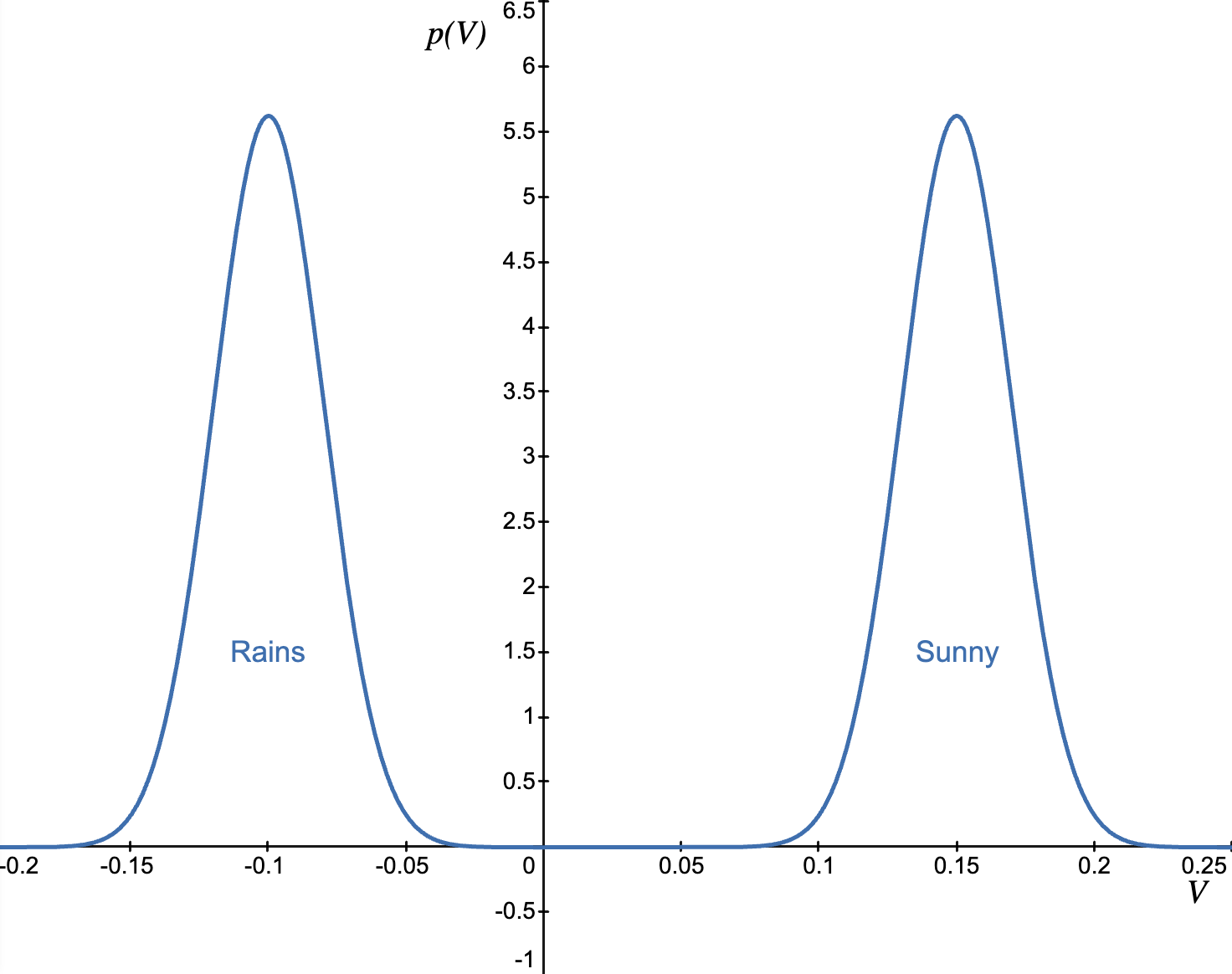
Consider a frame $\phi_{walk}$ of going out for a walk. You know there's 50% chance it will rain. Do you take the umbrella or not? You can imagine two counterfactuals: one where you take the umbrella, and one where you don't.

Below is the potential $p_{\phi_{walk}}(v)$ of the frame without the umbrella. We can see a bimodal distribution of Value outcomes. If it ends up raining, varying degrees of negative Value outcomes can be expected (getting wet, cold, ill), which is modeled by the left hump. The right hump models the distribution of expected positive outcomes when the weather is good.

For how to read this probability density function see Potential.

Now, if we consider taking the umbrella, $\phi_{walk}^{x}$, we might see potential like this:

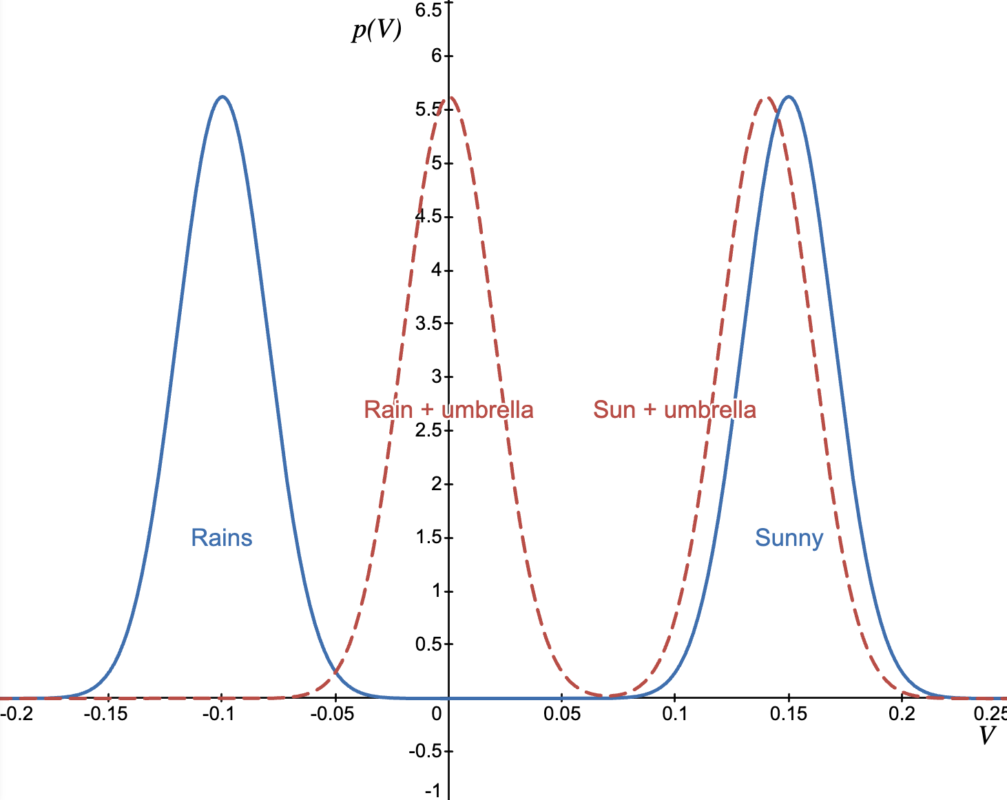
The "rainy weather" hump has moved to the right, which means that the negative Value outcomes of the rainy case have been mostly minimized. The second "good weather" hump has moved slightly to the left, because the carrying cost of umbrella introduces a slight drag in our walking frame. It's important to note that if umbrella had no carrying costs, we'd always take it with us, because there would be only an upside. That's similar to how we tend to take our smartphone with us everywhere we go, even if we don't need it in most cases. Because it fits in the pocket, the carrying cost is practically 0.

This difference between the two potentials is marginal potential. Phenomenologically, marginal potential is the felt difference between two counterfactual frames, and this difference is intuitively assigned or associated to the entities, which we're using to transform our frame. A “thing” $x$ transforms the frame (and thus the distribution) $p_\phi \to p_\phi^x$.

The question is whether the transformation is useful? Just by looking at the transformed shapes above it's not obvious which one is better. The shapes (and associated emotions) cannot simply be subtracted from one another. They have to be compared by an aspect that we find relevant. If the aspect that we're interested in is expected Value then we subtract expected Value of $p_\phi$ from $p_\phi^x$ and see if the result is positive.

But we're not merely rational agents that look only at expected Value, otherwise gambling and lotteries wouldn't exist. We can define a summary functional $A[\cdot]$ that encodes other aspects of the potential/feeling that we care about: risk-aversion, downside safety, etc. Just like expected Value, these operations pull out a numerical aspect from the distribution $p_\phi$ to afford a meaningful comparison between the two frames.

The marginal potential of $x$ in frame $\phi$, under $A$ functional, can be defined as:

$\boxed{P_\phi^A(x)=A\left[p_\phi^x\right]-A\left[p_\phi\right]},$

Humans don’t use the same rule everywhere. In safety-critical contexts we are tail-focused; in exploration we tolerate variance. $A$ lets the same formalism serve different aims. Because $A$ can be chosen to reflect what the frame cares about, $P_\phi^A(x)$ directly measures the meaningful contribution of $x$ (tool vs obstacle) in that context. If we care about trust or fear of ruin, we can compute the $P_\phi^A(x)$ under the right functional, and have a decision signal for whether to include $x$.

Here are some simple functionals:

• Expected value: $A_E=\int v\,p(v)\,dv$
  Measures the average gain/loss and assumes risk neutrality. Use for planning under mild risk when the mean is a sufficient summary; it ignores variance, tails, and multimodality.

• Trust coefficient: $A_T=\Pr(V>0)-\Pr(V<0)\in[-1,1]$
  Captures whether the distribution leans positive or negative, disregarding magnitudes. Good for quick go/no-go judgments and signaling “more good than bad branches,” but insensitive to how good or bad.

• Risk-averse utility: $A_u=\int u(v)\,p(v)\,dv$ with concave $u$
  Encodes diminishing returns and loss aversion via the shape of $u$. Choose $u$ to reflect the frame’s attitude to risk; if $u$ is linear, it reduces to expected value.